3D-Geo-Vis 2.0 – Methodology

Back to App

Introduction

This page documents the 3D geovisualization methods and graphic variables implemented in the 3D-Geo-Vis 2.0 application and is based on the article Zejdlik & Vozenilek (2025) Reference:
Zejdlik, J., & Vozenilek, V. (2025). Methods of 3D geovisualization of thematic data in the context of graphic variables. International Journal of Cartography, 0(0), 1–16. https://doi.org/10.1080/23729333.2025.2555508
.

3D Geovisualization Methods

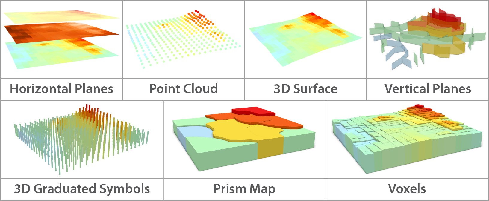
Graphic representation of seven selected methods
Graphic representation of seven selected methods of 3D geovisualization of thematic data

Horizontal Planes

Horizontal plane is a way of displaying raster spatial data where the entire dataset has a constant elevation (Z) coordinate and differs only in the way it is displayed, such as the color of the cell. Visualization of 2D planes in the form of static outputs is quite limiting, as they overlap when displaying multiple planes at different height levels. For this reason, it is desirable to use this type of visualization in an interactive environment, which is also necessary for visual analysis and data exploration (Zejdlik and Vozenilek, 2024) Reference:
Zejdlik, J., & Vozenilek, V. (2024). Evaluation of 3D geovisualization of volumetric geospatial data in the form of horizontal planes using selected software. Geographia Cassoviensis, 18(1), 5–25. https://doi.org/10.33542/GC2024-1-01
.

Horizontal Planes Visualization

Point Cloud

A point cloud is a type of discrete visualization where each point is represented by three coordinates. It can be a 2D point cloud, where all points have a constant Z coordinate, or a 3D point cloud, where the Z coordinate is variable. Point clouds can be distributed randomly or in a regular grid. Ideally, the user can dynamically change the size and density of the dots to achieve the best possible visual analysis (Gautier et al., 2020) Reference:
Gautier, J., Christophe, S., & Brédif, M. (2020). Visualizing 3D climate data in urban 3D models. ISPRS - International Archives of the Photogrammetry, Remote Sensing and Spatial Information Sciences, XLIII-B4-2020. https://doi.org/10.5194/isprs-archives-XLIII-B4-2020-781-2020
.

Point Cloud Visualization

3D Surface

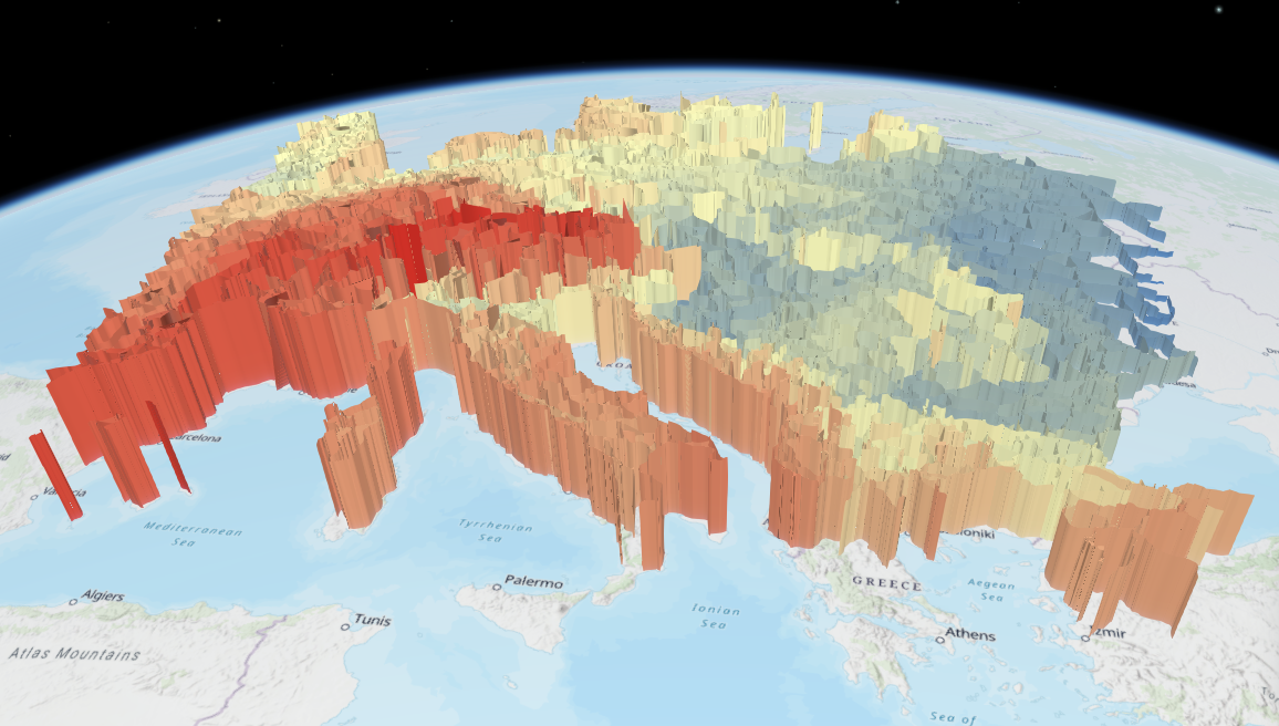
A 3D surface is a method of continuous visualization usually created by interpolating points from a point cloud. The pixel height (Z coordinate) is variable depending on the value of the phenomenon. 3D surfaces are most often used to represent elevation (digital elevation models), but they can also be used, for example, to represent socio-economic phenomena (so-called social or digital surfaces). Socioeconomic data have different characteristics than data from physical geography. Therefore, it is not enough to use the same methods and just change the data. It is always necessary to know the investigated phenomenon and adapt the visualization method to it (Jakobi and Nemes Nagy, 2006) References:
Jakobi, Á., & Nemes Nagy, J. (2006). Digital surface in social geography. Az Eötvös Loránd Tudományegyetem Térképtudományi És Geoinformatikai Tanszékének Évkönyve.
.

3D Surface

Vertical Planes

Vertical planes are usually located in the middle of urban roads and rendered by extruding vertically the linear geometry of the road network (Figure 5). In order to answer possible occlusion issues, transparency can be applied to the vertical planes (Gautier et al., 2020a) References:
Gautier, J., Christophe, S., & Brédif, M. (2020). Visualizing 3D climate data in urban 3D models. ISPRS - International Archives of the Photogrammetry, Remote Sensing and Spatial Information Sciences, XLIII-B4-2020. https://doi.org/10.5194/isprs-archives-XLIII-B4-2020-781-2020
. Jedlička et al. (2024) References:
Jedlička, K., Andrš, T., Čerba, O., Mildorf, T., Beran, D., Hájek, P., & Kepka, M. (2024). INTERACTIVE CARTOGRAPHY OF AIR QUALITY: A METHOD FOR TRAFFIC POLLUTION ANALYSIS. Proceedings, 9th International Conference on Cartography and GIS, 16-21 June 2024, Nessebar, Bulgaria, 373–385.
refer to the method as 3D Flow Map, which is based on Flow Map – a method of thematic cartography used for the expression of linear phenomenon with quantitative or qualitative attributes alongside the geometry of the line.

Vertical Planes

3D Graduated Symbols

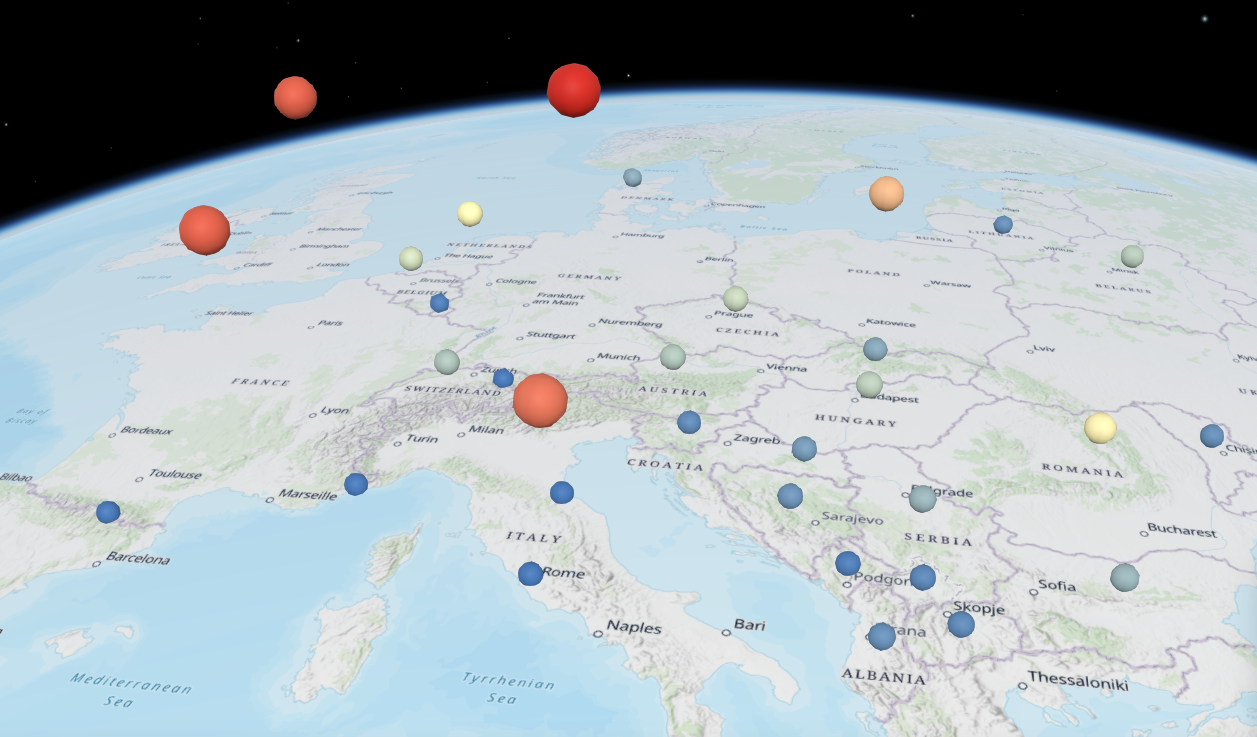
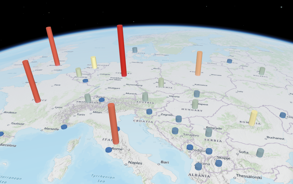
This method is based on 2D graduated symbols method used in thematic maps. Symbols can take many forms, from 3D bars to spheres to pie charts, while the size of these elements depends on the value (eg column height, sphere diameter). Testing suitable representations of quantitative spatial data in 3D virtual environments using 3D graduated symbols was dealt with by Bleisch (2011) References:
Bleisch, S. (2011). Toward Appropriate Representations of Quantitative Data in Virtual Environments. Cartographica, 46, 252–261. https://doi.org/10.3138/carto.46.4.252
. Six potentially appropriate proportional symbols for the display of quantitative data in virtual environments were experimentally tested: 2D bars, 3D bars, and 2D circles, with and without reference frames indicating the largest possible value (Bleisch, 2011) References:
Bleisch, S. (2011). Toward Appropriate Representations of Quantitative Data in Virtual Environments. Cartographica, 46, 252–261. https://doi.org/10.3138/carto.46.4.252
. Stoter et al. (2008) References:
Stoter, J., de Kluijver, H., & Kurakula, V. (2008). 3D noise mapping in urban areas. International Journal of Geographical Information Science, 22(8), 907–924. https://doi.org/10.1080/13658810701739039
used 3D graduated symbols to visualize the noise level using so-called virtual microphones. A virtual microphone, specified with x, y, z coordinates, is a point that reports what the noise level would be at a certain location under given circumstances.

3D Graduated Symbols

Prism Map

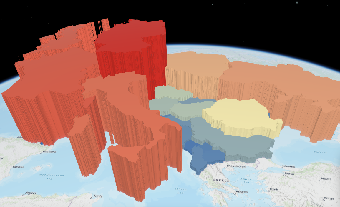
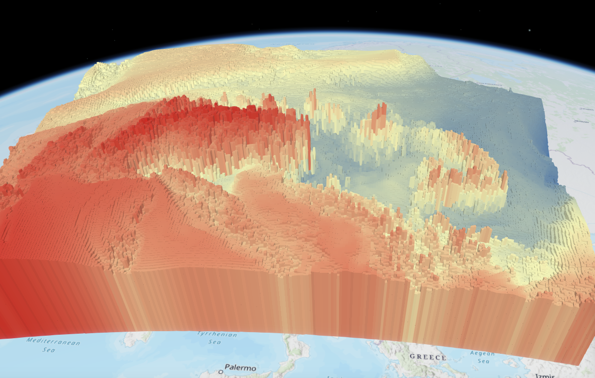
A prism map is a 3D choropleth map with extruded height to encode a numerical attribute. Prism maps are predominantly used for visual impact, and the unfamiliarity with prism maps hampers their understanding (Field, 2018) References:
Field, K. (2018). Cartography. (1st ed.). Esri Press. ISBN 978-1-58948-439-9
. Height (the visual variable used by prism maps) is far more accurate for interpreting associated quantitative values than brightness (the visual variable commonly used by choropleth maps), but perspective foreshortening and oblique viewing angles can result in distortion and excessive occlusion in prism maps (Cleveland and McGill, 1984) References:
Cleveland, W. S., & McGill, R. (1984). Graphical Perception: Theory, Experimentation, and Application to the Development of Graphical Methods. Journal of the American Statistical Association, 79(387), 531–554. https://doi.org/10.1080/01621459.1984.10478080
.

Prism Map

Voxels

In geovisualization using voxels, the data is represented by blocks with different heights depending on their values. It has common elements with a 3D graduated symbols and prism map. Unlike 3D graduated symbols, in the case of voxels, adjacent blocks (voxels) are connected to each other, and unlike a prism map, all polygons have the same size. Rae (2016) References:
Rae, A. (2016). The Global Human Settlement Layer: An amazing new global population dataset. http://www.statsmapsnpix.com/2016/10/the-global-human-settlement-layer.html
used The Global Human Settlement Layer data to represent population in selected cities using voxels. His approach was applied in 2018 by The Pudding to create an interactive web map application, using the same dataset to represent population for the entire world (The Pudding, 2024) References:
The Pudding. (2024). Human Terrain. https://pudding.cool/2018/10/city_3d
.

Voxels

Graphic Variables

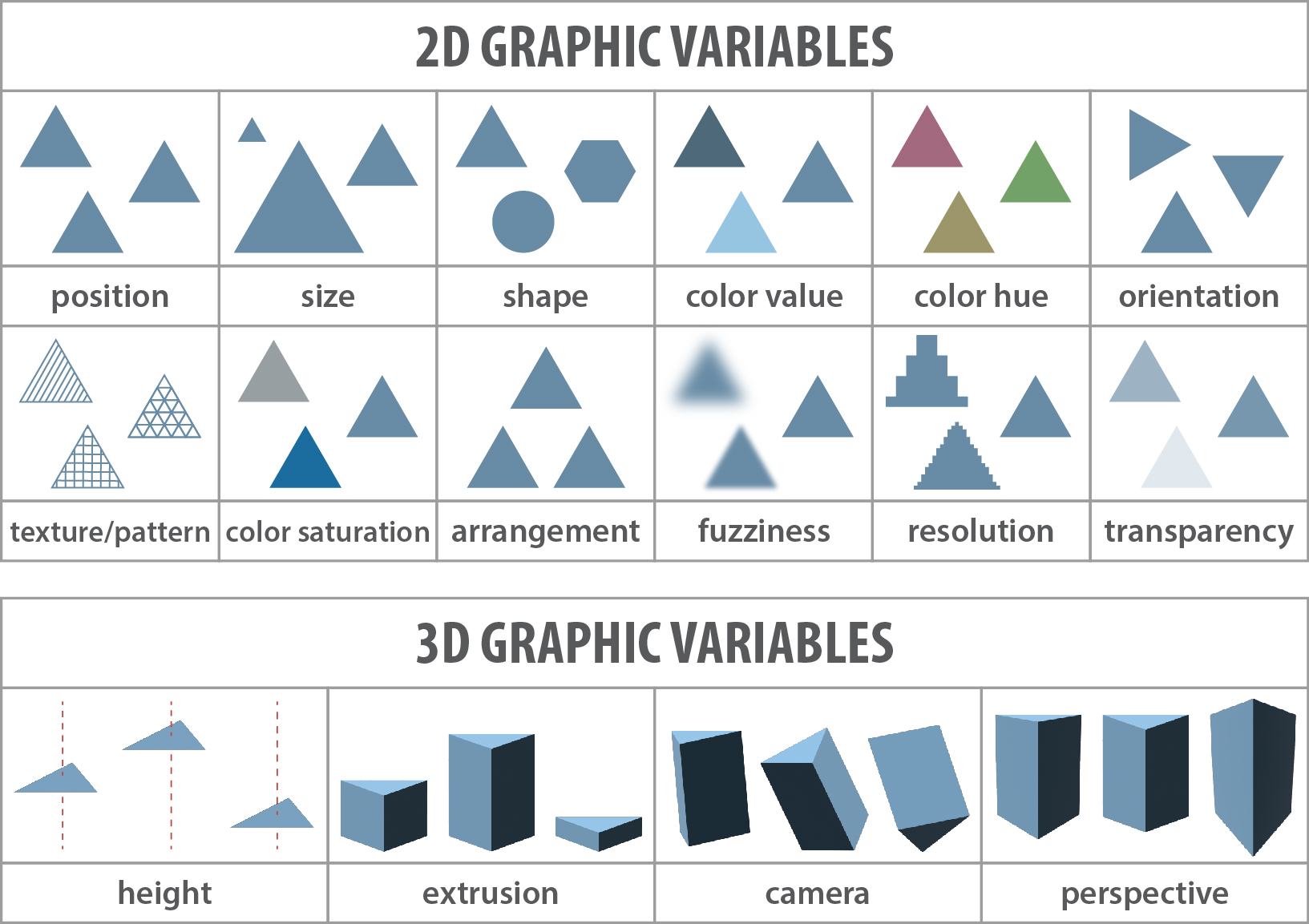
Graphic variables selected for evaluation
Graphic variables selected for evaluation of methods of 3D geovisualization of thematic data

2D Graphic Variables

Graphic or visual variables describe the graphic dimensions in which a map or other visualization can be changed to encode information. Graphic variables are differences in map elements perceived by the human eye. Regardless of the type of map, these are basic ways of distinguishing graphic symbols (Axis Maps, 2023) Reference:
Axis Maps. (2023). Visual Variables. Cartography Guide - A Short, Friendly Guide to Basic Principles of Map Design. https://www.axismaps.com//guide/visual-variables
. For example, Garlandini and Fabrikant (2009) Reference:
Garlandini, S., & Fabrikant, S. I. (2009). Evaluating the Effectiveness and Efficiency of Visual Variables for Geographic Information Visualization. In K. S. Hornsby, C. Claramunt, M. Denis, & G. Ligozat (Eds.), Spatial Information Theory (pp. 195–211). Springer. https://doi.org/10.1007/978-3-642-03832-7_12
dealt with the evaluation of the effectiveness and efficiency of visual variables for the visualization of geographic information. Visual variables were originally described by the French cartographer Jacques Bertin (1918–2010) in the book Sémiologie Graphique (Semiology of Graphics) in the original 1967 edition, revised in 1983 (Roth, 2017) Reference:
Roth, R. E. (2017). Visual Variables. In International Encyclopedia of Geography (pp. 1–11). John Wiley & Sons, Ltd. https://doi.org/10.1002/9781118786352.wbieg0761
. The original so-called "retinal variables" (Bertin, 1967) Reference:
Bertin, J. (1967). Sémiologie graphique: Les diagrammes, les réseaux, les cartes. Gauthier-Villars.
included:

  • position (the location of a symbol on the map);
  • size (the relative dimension of a symbol);
  • shape (the geometric form of a symbol);
  • color value (variation from light to dark);
  • color hue (variation in color type);
  • orientation (directional rotation of a symbol);
  • texture/pattern (surface fill variation).

This list was then gradually expanded by other cartographers (MacEachren, 2004 Reference:
MacEachren, A. M. (2004). How Maps Work: Representation, Visualization, and Design (1st edition). The Guilford Press.
; Morrison, 1974 Reference:
Morrison, J. L. (1974). A theoretical framework for cartographic generalization with the emphasis on the process of symbolization. International Yearbook of Cartography, 14(1974), 115–127.
; Roth, 2017) Reference:
Roth, R. E. (2017). Visual Variables. In International Encyclopedia of Geography (pp. 1–11). John Wiley & Sons, Ltd. https://doi.org/10.1002/9781118786352.wbieg0761
:

  • color saturation (the intensity of color);
  • arrangement (the spatial organization of elements);
  • crispness/fuzziness (sharp vs. blurred boundaries);
  • resolution (the level of detail);
  • transparency (the degree of opacity).

3D Graphic Variables

In addition, the 3D environment allows the evaluation of other graphic variables, such as perspective, camera, lighting, shading, atmospheric effects (Krejčí, 2018) Reference:
Krejčí, M. (2018). Dynamické grafické proměnné ve 3D mapách [Diplomová práce, Masarykova univerzita, Přírodovědecká fakulta]. https://theses.cz/id/35lr4j/
, height, extrusion, object surface (pattern, shading), light emission (Limberger et al., 2023) Reference:
Limberger, D., Scheibel, W., Döllner, J., & Trapp, M. (2023). Visual variables and configuration of software maps. Journal of Visualization, 26(1), 249–274. https://doi.org/10.1007/s12650-022-00868-1
or fog (Vetter, 2023) Reference:
Vetter, M. (2023). The usage of “fog” as a visual variable in 3D-cartographic virtual reality environments. Abstracts of the ICA, 6, 1–2. https://doi.org/10.5194/ica-abs-6-263-2023
. For the purposes of this paper, four 3D graphic variables were selected to evaluate 3D geovisualization methods, namely:

  • height (vertical dimension of the symbol);
  • extrusion (expansion of a 2D object into the third dimension);
  • camera / point of view (the place from which the user looks at the object or scene);
  • perspective (the way an object or scene is rendered to appear realistic in terms of depth and space).